Lighthouse Labs W7D5 - Pipelines and Model Persistence Instructor: Socorro E. Dominguez-Vidana

Overview - Pipelines

• [] Motivation and example
• [] Feature unions
• [] Column transformers
• [] Visualizing pipelines
• [] Hyperparameter tuning with pipelines
• [] Custom class in a pipeline

Mario and Luigi have been hired to get water flowing smoothly through a set of pipes. Each part of the job has to be done in the right order, and they use their plumbing pipeline to keep it organized.

1. Clear the Pipes Luigi goes first, clearing out any clogs and making sure the pipes are clean. In a ML pipeline, this is like cleaning the data

2. Check the Pipe Sizes Next, Mario measures and standardizes the pipes to ensure they're compatible. This step would be similar to scaling or normalizing the data.

3. Install Filters To keep the water clean, Luigi adds filters at specific points in the pipeline. Similarly, we may add steps to transform data or select only the features we need, so only relevant information goes through.

4. Test the Water Flow Before they finish, Mario and Luigi test the water flow to make sure everything works. In ML, this step is like training and testing a model guaranteeing that our setup can handle real-world data.

5. Final Check and Save the Setup Finally, they document how they set up the pipes so anyone can understand it if they need repairs later. In ML, we can save the pipeline model with joblib or pickle so we can use it again without setting it up from scratch.

Why Use a Pipeline?

• Reuse steps easily for new data.
• Test everything consistently and know the exact order, so there are no surprises in model performance.

In simple terms, an ML pipeline is our plumbing plan for handling data from start to finish, making sure every step flows correctly.

Using pipelines

Besides being a plumber, Mario took up another role: Doctor Mario!

The famous plumber-turned-physician is on a new mission: tackling diabetes! In his clinic, he got access to the diabetes dataset that holds information on patients' age, blood pressure, BMI, and more. With this data, Dr. Mario can identify risk factors, predict who might be at risk, and create better treatment plans.

Just like fixing a tricky pipe, understanding diabetes requires the right tools and steps.

import pandas as pd

df = pd.read_csv('data/diabetes.csv')
df.head()

	preg	plas	pres	skin	test	mass	pedi	age	class
0	6	148	72	35	0	33.6	0.627	50	1
1	1	85	66	29	0	26.6	0.351	31	0
2	8	183	64	0	0	23.3	0.672	32	1
3	1	89	66	23	94	28.1	0.167	21	0
4	0	137	40	35	168	43.1	2.288	33	1

from sklearn.model_selection import train_test_split
from sklearn.preprocessing import StandardScaler
from sklearn.decomposition import PCA
from sklearn.linear_model import LogisticRegression, RidgeClassifier
from sklearn.metrics import accuracy_score

Without a Pipeline

X = df.drop(columns='class')
y = df['class']

X_train, X_test, y_train, y_test = train_test_split(X, y, test_size=0.2, random_state=27, stratify=y)

scaler = StandardScaler()
scaler.fit(X_train)
X_train_scaled = scaler.transform(X_train)

pca = PCA(n_components=3)
pca.fit(X_train_scaled)
X_train_pca = pca.transform(X_train_scaled)

model = LogisticRegression()
model.fit(X_train_pca, y_train)

# Test portion
X_test_scaled = scaler.transform(X_test)
X_test_pca = pca.transform(X_test_scaled)

y_pred = model.predict(X_test_pca)
acc = accuracy_score(y_test, y_pred)
print(f'Test set accuracy: {acc}')

Test set accuracy: 0.6948051948051948

There are several inconvenient things about this: then our model will not work as expected.

1. We have a lot of ugly code. We keep calling .fit() and .transform() on different objects, and we keep having to rename transformed variables so as not to cause confusions later in our notebook.
2. Our preprocessing and modeling code is distributed and therefore error-prone. If we try running our model somewhere else and forget to copy over a step (e.g. we don't apply StandardScaler to the test set),

3. We can only use convenient Sklearn functions/classes such as GridSearchCV() on the model class (e.g. LogisticRegression). What if we want to try different numbers of components, or different scaling methods?

The solution: Sklearn Pipelines

from sklearn.pipeline import Pipeline

pipeline = Pipeline(steps=[('scaling', StandardScaler()),
                           ('pca', PCA(n_components=3)),
                           ('classifier', LogisticRegression())])
pipeline.fit(X_train, y_train)

y_pred = pipeline.predict(X_test)
acc = accuracy_score(y_test, y_pred)
print(f'Test set accuracy: {acc}')

Test set accuracy: 0.6948051948051948

Notice how much cleaner this code is. The composite model created using Pipeline can be used just like any other Sklearn model you have learned, which means that it can also be passed to functions like cross_val_score().

---

Feature unions

Pipeline lets us specify a sequence of steps that will be executed in one after the other (i.e. in series). But it wouldn't make sense if Mario always had to wait for Luigi to finish a job. Sometimes, Mario and Luigi can each work on different parts of a job at the same time, then combining their results at the end.

In ML, sometimes we want to apply different transformations to our data in parallel and then combine the results. We might want to scale numerical features (like age or pregnancies) while applying one-hot encoding to categorical features (like gender or city). Instead of doing this in separate steps, FeatureUnion lets us do both at once and then joins them together. FeatureUnion's can be composed with Pipeline's however much we want.

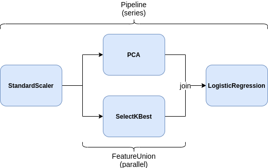
from sklearn.pipeline import FeatureUnion
from sklearn.feature_selection import SelectKBest

feature_union = FeatureUnion([('pca', PCA(n_components=3)), 
                              ('select_best', SelectKBest(k=6))])

pipeline = Pipeline(steps=[('scaling', StandardScaler()),
                           ('features', feature_union),
                           ('classifier', LogisticRegression())])
pipeline.fit(X_train, y_train)

y_pred = pipeline.predict(X_test)
acc = accuracy_score(y_test, y_pred)
print(f'Test set accuracy: {acc}')

Test set accuracy: 0.7337662337662337

---

Column transformers

FeatureUnion doesn’t automatically "split" the data between transformers. It applies each transformer to the full dataset. For different transformations applied to specific parts of the data, we use ColumnTransformer, which allows you to specify which columns should go to which transformation.

For instance, for a dataset with both numerical and categorical features, we may want to do something like the following:

1. For numeric columns:
   1. Impute missing values with the mean
   2. Standard scale the values
2. For categorical columns:
   1. Impute missing values with the mode
   2. One-hot-encode the categories
3. Fit a model to the resulting features

ColumnTransformer has a very similar syntax to that of a FeatureUnion or Pipeline, except that we must also specify the column names that each transform applies to.

Doctor Mario is tackling heart disease now! With patient data on age, cholesterol, heart rate, and more, he aims to identify key risk factors to help his patients.

Feature	Description
age	Age of the patient in years
sex	Sex of the patient (1 = male, 0 = female)
cp	Chest pain type (0: typical angina, 1: atypical angina, 2: non-anginal pain, 3: asymptomatic)
trestbps	Resting blood pressure in mm Hg
chol	Serum cholesterol in mg/dl
fbs	Fasting blood sugar > 120 mg/dl (1 = true, 0 = false)
restecg	Resting electrocardiographic results (0: normal, 1: ST-T wave abnormality, 2: probable left ventricular hypertrophy)
thalach	Maximum heart rate achieved
exang	Exercise-induced angina (1 = yes, 0 = no)
oldpeak	ST depression induced by exercise relative to rest
slope	Slope of the peak exercise ST segment (0: upsloping, 1: flat, 2: downsloping)
ca	Number of major vessels (0-3) colored by fluoroscopy
thal	Thalassemia (3 = normal, 6 = fixed defect, 7 = reversible defect)
target	Diagnosis of heart disease (1 = disease, 0 = no disease)

df = pd.read_csv('data/heart_disease.csv')
df.head()

	age	sex	cp	trestbps	chol	fbs	restecg	thalach	exang	oldpeak	slope	ca	thal	target
0	63.0	1.0	1.0	145.0	233.0	1.0	2.0	150.0	0.0	2.3	3.0	0.0	6.0	0
1	67.0	1.0	4.0	160.0	286.0	0.0	2.0	108.0	1.0	1.5	2.0	3.0	3.0	2
2	67.0	1.0	4.0	120.0	229.0	0.0	2.0	129.0	1.0	2.6	2.0	2.0	7.0	1
3	37.0	1.0	3.0	130.0	250.0	0.0	0.0	187.0	0.0	3.5	3.0	0.0	3.0	0
4	41.0	0.0	2.0	130.0	204.0	0.0	2.0	172.0	0.0	1.4	1.0	0.0	3.0	0

X, y = df.drop(columns='target'), df['target'].values
X_train, X_test, y_train, y_test = train_test_split(X, y, random_state=27)

from sklearn.compose import ColumnTransformer
from sklearn.preprocessing import OneHotEncoder
from sklearn.impute import SimpleImputer

numerical_features = ["age", "trestbps", "chol", "thalach", "oldpeak"]
categorical_features = ["sex", "cp", "fbs", "restecg", "exang", "slope", "ca", "thal"]

numeric_transform = StandardScaler()
categorical_transform = OneHotEncoder(handle_unknown="ignore")

preprocessor = ColumnTransformer([('numeric', numeric_transform, numerical_features), 
                                  ('categorical', categorical_transform, categorical_features)])

pipeline = Pipeline(steps=[
    ("preprocessor", preprocessor),
    ("classifier", LogisticRegression())
])
                     
pipeline.fit(X_train, y_train)

Pipeline(steps=[('preprocessor',
                 ColumnTransformer(transformers=[('numeric', StandardScaler(),
                                                  ['age', 'trestbps', 'chol',
                                                   'thalach', 'oldpeak']),
                                                 ('categorical',
                                                  OneHotEncoder(handle_unknown='ignore'),
                                                  ['sex', 'cp', 'fbs',
                                                   'restecg', 'exang', 'slope',
                                                   'ca', 'thal'])])),
                ('classifier', LogisticRegression())])

In a Jupyter environment, please rerun this cell to show the HTML representation or trust the notebook.
On GitHub, the HTML representation is unable to render, please try loading this page with nbviewer.org.

What is the ColumnTransformer actually doing? We can get a better sense by looking at our data before and after the transform it applies.

from sklearn.metrics import accuracy_score
y_pred = pipeline.predict(X_test)

acc = accuracy_score(y_test, y_pred)
print(f"Test set accuracy: {acc}")

Test set accuracy: 0.618421052631579

# Initial data
X.head()

	age	sex	cp	trestbps	chol	fbs	restecg	thalach	exang	oldpeak	slope	ca	thal
0	63.0	1.0	1.0	145.0	233.0	1.0	2.0	150.0	0.0	2.3	3.0	0.0	6.0
1	67.0	1.0	4.0	160.0	286.0	0.0	2.0	108.0	1.0	1.5	2.0	3.0	3.0
2	67.0	1.0	4.0	120.0	229.0	0.0	2.0	129.0	1.0	2.6	2.0	2.0	7.0
3	37.0	1.0	3.0	130.0	250.0	0.0	0.0	187.0	0.0	3.5	3.0	0.0	3.0
4	41.0	0.0	2.0	130.0	204.0	0.0	2.0	172.0	0.0	1.4	1.0	0.0	3.0

# Preprocessed data
X_preprocessed = preprocessor.transform(X)
X_preprocessed[0]

array([ 0.92303809,  0.78129791, -0.2614227 ,  0.08134766,  1.07875303,
        0.        ,  1.        ,  1.        ,  0.        ,  0.        ,
        0.        ,  0.        ,  1.        ,  0.        ,  0.        ,
        1.        ,  1.        ,  0.        ,  0.        ,  0.        ,
        1.        ,  1.        ,  0.        ,  0.        ,  0.        ,
        0.        ,  0.        ,  1.        ,  0.        ,  0.        ])

---

Visualizing pipelines

Another advantage of having these pipelines is that we can quickly visualize complex workflows used in our modeling as HTML, which can be helpful for debugging purposes or presentations.

_{Note: I highly recommend you use this in your own presentations as a substitute for (or in addition to) code.}

# Display HTML representation in a jupyter context
from sklearn import set_config
set_config(display='diagram')

pipeline

Pipeline(steps=[('preprocessor',
                 ColumnTransformer(transformers=[('numeric', StandardScaler(),
                                                  ['age', 'trestbps', 'chol',
                                                   'thalach', 'oldpeak']),
                                                 ('categorical',
                                                  OneHotEncoder(handle_unknown='ignore'),
                                                  ['sex', 'cp', 'fbs',
                                                   'restecg', 'exang', 'slope',
                                                   'ca', 'thal'])])),
                ('classifier', LogisticRegression())])

In a Jupyter environment, please rerun this cell to show the HTML representation or trust the notebook.
On GitHub, the HTML representation is unable to render, please try loading this page with nbviewer.org.

Note that you can also click on the individual parts in the diagram (e.g. StandardScaler) to see their arguments.

# Or, save the HTML to a file
from sklearn.utils import estimator_html_repr

with open('img/model_pipeline.html', 'w') as f:  
    f.write(estimator_html_repr(pipeline))

---

Hyperparameter tuning with pipelines

Normally, if we want to tune hyperparameters using something like GridSearchCV, we need to pass it: A model object. A dictionary of (parameter name, list of values to try) pairs. When not using pipelines, we can only tune hyperparameters for a single model (the one we specify as the model in GridSearchCV. As we've seen, however, we can create composite models using Pipeline. We can then pass this composite model to GridSearchCV and tune hyperparameters for multiple components at once.

from sklearn.model_selection import GridSearchCV, cross_val_score

pipeline = Pipeline(steps=[
    ('imputer', SimpleImputer(strategy='mean')),
    ('scaling', StandardScaler()),
    ('pca', PCA()),
    ('classifier', LogisticRegression())
])

# Define the parameter grid
param_grid = {
    'pca__n_components': [2, 3, 4],
    'classifier__C': [0.1, 1, 10, 100],
    'classifier__solver': ['liblinear', 'lbfgs']}

# GridSearchCV with cross-validation
grid_search = GridSearchCV(estimator=pipeline, param_grid=param_grid, cv=5, scoring='accuracy')
grid_search.fit(X_train, y_train)

print(f'Best Parameters: {grid_search.best_params_}')
print(f'Best Cross-Validation Score: {grid_search.best_score_}')

# Evaluate the test set with the best model found
best_pipeline = grid_search.best_estimator_
acc = best_pipeline.score(X_test, y_test)
print(f'Test set accuracy with best parameters: {acc}')

Best Parameters: {'classifier__C': 0.1, 'classifier__solver': 'liblinear', 'pca__n_components': 3}
Best Cross-Validation Score: 0.6125603864734299
Test set accuracy with best parameters: 0.5921052631578947

In addition to trying out different hyperparameters for a given step in the pipeline, you can also try different classes altogether. For instance, what if we wanted to try both Logistic Regression and SVM for the "classifier" step?

from sklearn.svm import SVC

pipeline = Pipeline([
    ('imputer', SimpleImputer(strategy='mean')), 
    ('scaler', StandardScaler()),
    ('pca', PCA()),
    ('classifier', LogisticRegression())  # Placeholder for classifier
])

param_grid = [
    {
        'pca__n_components': [2, 3, 4],
        'classifier': [LogisticRegression()],
        'classifier__C': [0.1, 1, 10, 100],
        'classifier__solver': ['liblinear', 'lbfgs']
    },
    {
        'pca__n_components': [2, 3, 4],
        'classifier': [SVC()],
        'classifier__C': [0.1, 1, 10, 100],
        'classifier__kernel': ['linear', 'rbf']
    },
    {
        'pca__n_components': [2, 3, 4],
        'classifier': [RidgeClassifier()],
        'classifier__alpha': [0.1, 0.01, 1.0]
    }
]


grid_search = GridSearchCV(pipeline, param_grid, cv=5, scoring='accuracy')
grid_search.fit(X_train, y_train)

GridSearchCV(cv=5,
             estimator=Pipeline(steps=[('imputer', SimpleImputer()),
                                       ('scaler', StandardScaler()),
                                       ('pca', PCA()),
                                       ('classifier', LogisticRegression())]),
             param_grid=[{'classifier': [LogisticRegression()],
                          'classifier__C': [0.1, 1, 10, 100],
                          'classifier__solver': ['liblinear', 'lbfgs'],
                          'pca__n_components': [2, 3, 4]},
                         {'classifier': [SVC()],
                          'classifier__C': [0.1, 1, 10, 100],
                          'classifier__kernel': ['linear', 'rbf'],
                          'pca__n_components': [2, 3, 4]},
                         {'classifier': [RidgeClassifier()],
                          'classifier__alpha': [0.1, 0.01, 1.0],
                          'pca__n_components': [2, 3, 4]}],
             scoring='accuracy')

In a Jupyter environment, please rerun this cell to show the HTML representation or trust the notebook.
On GitHub, the HTML representation is unable to render, please try loading this page with nbviewer.org.

print("Best Parameters:", grid_search.best_params_)
print("Best Cross-Validation Score:", grid_search.best_score_)

Best Parameters: {'classifier': SVC(), 'classifier__C': 10, 'classifier__kernel': 'rbf', 'pca__n_components': 2}
Best Cross-Validation Score: 0.6302415458937198

y_pred = grid_search.best_estimator_.predict(X_test)
acc = accuracy_score(y_test, y_pred)
print(f"Test set accuracy: {acc}")

Test set accuracy: 0.5921052631578947

Model Persistence

After hours of fixing pipes, Mario and Luigi don't want to start from scratch if they have to revisit the job. In ML, pipelines can take a long time to .fit, and you will not want to run the whole notebook every single time - we want to save the model so we can use it again without retraining.

This process is called model persistence. Just like Mario and Luigi might record their work notes, we use pickle or joblib to save models. This lets us load them back up later ready to make predictions.

---

Serialization is the process of converting a program entity into a stream of bytes that can be saved as a file. Serialization:

• Avoids redundant training. Models can take a long time to train and data can take a long time to load/process
• allows us to deploy the model into an application.

---

Pickle

• Pickling is the process where a Python object is converted into a byte stream (usually not human readable).
• Unpickling is the reverse operation, where a byte stream is converted back into a working Python object.
• Pickling is the simplest way to store the object from a coding perspective.
• The Python Pickle module is an object-oriented way of storing objects.
  • It can store any Python object, not just Sklearn models.

Features

• Store/load dictionaries and lists.
• Store/load the attributes of arbitrary data types (i.e. classes)
• Do this recursively, so that if your object has attributes that are classes themselves, it can be saved just as easily

Limitations

• Does not save the code of an object — only its attribute values.
• Cannot save file handles or connection sockets.
• Pickle is version-dependent. For example, if you saved a model with a certain version of Sklearn then try to load it with a different one (e.g. you updated), there may be issues.
  • Another motivation for using virtual environments, which can be containerized.

Saving procedure

import pickle        # Built-in python module

# Create some object and manipulate it in some way (e.g. train the model)
myobj = SomeClass(...)
myobj = myobj.some_method(...)

# Save to a file using Pickle
with open('myfile.pickle', 'wb') as file_handle:
    pickle.dump(myobj, file_handle)

Loading procedure

import pickle        # Built-in python module

# Load from a file using Pickle
with open('myfile.pickle', 'rb') as file_handle:
    myobj = pickle.load(file_handle)    # myobj will be an instance of SomeClass

Methods

The pickle module provides four different methods:

• dump() − The dump() method serializes to an open file (file-like object).
• dumps() − Serializes to a string.
• load() − Deserializes from an open-like object.
• loads() − Deserializes from a string.

Example

import pickle 

# Save the model
with open('saved_models/pipeline.pickle', 'wb') as f:
    pickle.dump(pipeline, f)

# Load the model
with open('saved_models/pipeline.pickle', 'rb') as f:
    pipeline_loaded = pickle.load(f)

pipeline_loaded

Pipeline(steps=[('imputer', SimpleImputer()), ('scaler', StandardScaler()),
                ('pca', PCA()), ('classifier', LogisticRegression())])

In a Jupyter environment, please rerun this cell to show the HTML representation or trust the notebook.
On GitHub, the HTML representation is unable to render, please try loading this page with nbviewer.org.

---

Joblib

Joblib is an alternative serialization module to Pickle. However, starting with Python 3.8, Pickle is actually better than Joblib for saving numpy arrays.
_{If you have Python >=3.8, just use Pickle. Source.*}

Saving procedure

import joblib

# Create some object and manipulate it in some way (e.g. train the model)
myobj = SomeClass(...)
myobj = myobj.some_method(...)

# Save to a file using Joblib
joblib.dump(myobj, file_path)

Loading procedure

import joblib

# Load from a file using Joblib
myobj = joblib.load(file_path)    # myobj will be an instance of SomeClass

Example

import joblib

joblib.dump(grid_search, 'saved_models/pipeline.can')

# Load the model
pipeline_loaded = joblib.load('saved_models/pipeline.can')

pipeline_loaded

GridSearchCV(cv=5,
             estimator=Pipeline(steps=[('imputer', SimpleImputer()),
                                       ('scaler', StandardScaler()),
                                       ('pca', PCA()),
                                       ('classifier', LogisticRegression())]),
             param_grid=[{'classifier': [LogisticRegression()],
                          'classifier__C': [0.1, 1, 10, 100],
                          'classifier__solver': ['liblinear', 'lbfgs'],
                          'pca__n_components': [2, 3, 4]},
                         {'classifier': [SVC()],
                          'classifier__C': [0.1, 1, 10, 100],
                          'classifier__kernel': ['linear', 'rbf'],
                          'pca__n_components': [2, 3, 4]},
                         {'classifier': [RidgeClassifier()],
                          'classifier__alpha': [0.1, 0.01, 1.0],
                          'pca__n_components': [2, 3, 4]}],
             scoring='accuracy')

In a Jupyter environment, please rerun this cell to show the HTML representation or trust the notebook.
On GitHub, the HTML representation is unable to render, please try loading this page with nbviewer.org.