Lighthouse Labs W4D5 - Introduction to Machine Learning (ML) Instructor: Socorro E. Dominguez-Vidana

Overview:

• [] Machine Learning
  • [] Supervised vs. Unsupervised Learning
• [] Supervised Learning
  • [] X and y
  • [] Regression vs. Classification
  • [] The golden rule: train/test split
• [] Simple Linear Regression
• [] Polynomial Regression

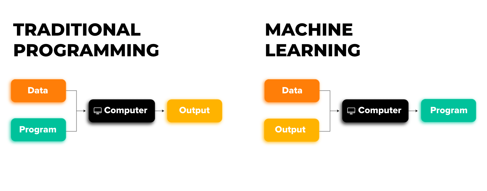
Machine Learning

What is Machine Learning (ML)?

• A subset of Artificial Intelligence.
• ML algorithms learn from data (training data) to make predictions or decisions without explicit programming.
• Models are built based on sample data to adapt and improve over time.

  “The field of study that gives computers the ability to learn without being explicitly programmed.” — Arthur Samuel (1959)

Types of Machine Learning

Supervised Learning

• Involves training models using labeled data, where the correct output is known. The algorithm learns to map inputs (X) to the desired outputs (y)

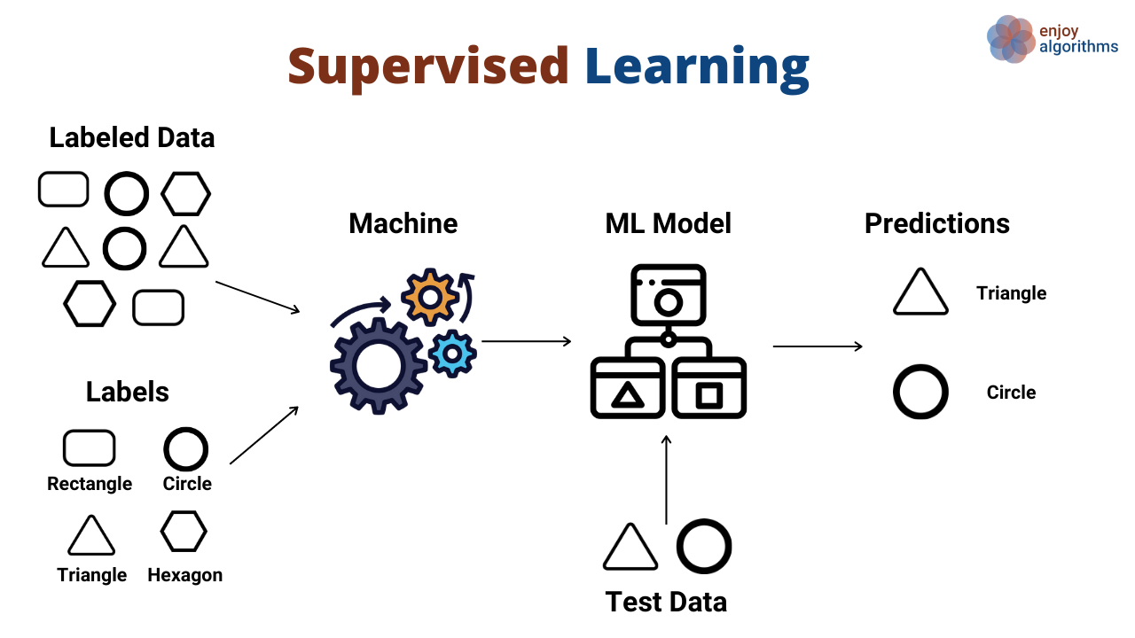
Author unknown. (n.d.). Supervised vs Unsupervised Machine Learning Medium.

Unsupervised Learning

• Works with unlabeled data, where the algorithm explores patterns and structures within the data without knowing the correct answers.

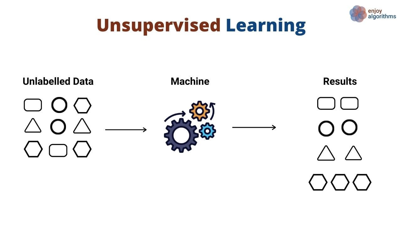
Author unknown. (n.d.). Data Science vs. Machine Learning Medium.

Supervised Learning: Regression & Classification

Classification Problems

• Classification is about assigning items to specific categories or groups, also called classes.
• The goal is to predict which class an input belongs to, based on patterns in the data.
  • Binary Classification: Involves two possible outcomes.
    • Predicting whether a patient has liver disease or not.
  • Multi-class Classification: Involves more than two classes.
    • Predicting a student’s letter grade (A, B, C, D, or F).
• Real-world applications:
  • Spam detection in emails (classify as spam or not spam).
  • Image recognition (classify objects or people in a photo).
  • Sentiment analysis (classify text as positive, negative, or neutral).

Regression Problems

• Regression is used when the task is to predict a continuous value rather than a discrete category.
• The goal is to model the relationship between the input variables and the output to make numerical predictions.
  • Linear Regression: The relationship between input features and the predicted value is modeled as a straight line.
    • Predicting house prices based on features like square footage, number of bedrooms, or location.
  • Non-linear Regression: The relationship is more complex and doesn’t follow a straight line.
    • Predicting the growth of a population over time.
• Real-world applications:
  • Forecasting stock prices based on historical data.
  • Predicting the amount of rainfall based on weather conditions like temperature and humidity.

Mukherjee, A. (n.d.). AI Part 3: Regression vs Classification Models. LinkedIn

The Golden Rule of Supervised Learning

• Once you've identified your features (X) and target (y), it's crucial to split your data into two sets: training and testing.

• You should only work with the training data when building your model.

  • If you involve test data in your decision-making (e.g., selecting or dropping features), you're allowing the test set to influence your choices.
  • This can cause data leakage, meaning your model has been indirectly exposed to the test data.
  • As a result, your model's performance won't reflect how it would perform on unseen data in real-world scenarios.

By keeping the test data untouched, your evaluation will be more reliable and representative of how the model generalizes to new data.

Training vs. Test Scores

• When evaluating a model, we typically look at two scores: training score vs. test score.
• The test score is more important because it reflects how the model performs on unseen data.
• Good models that generalize well will have similar training and test scores.
• Our goal is to choose models that can generalize well to new, unseen data, not just memorize the training data.

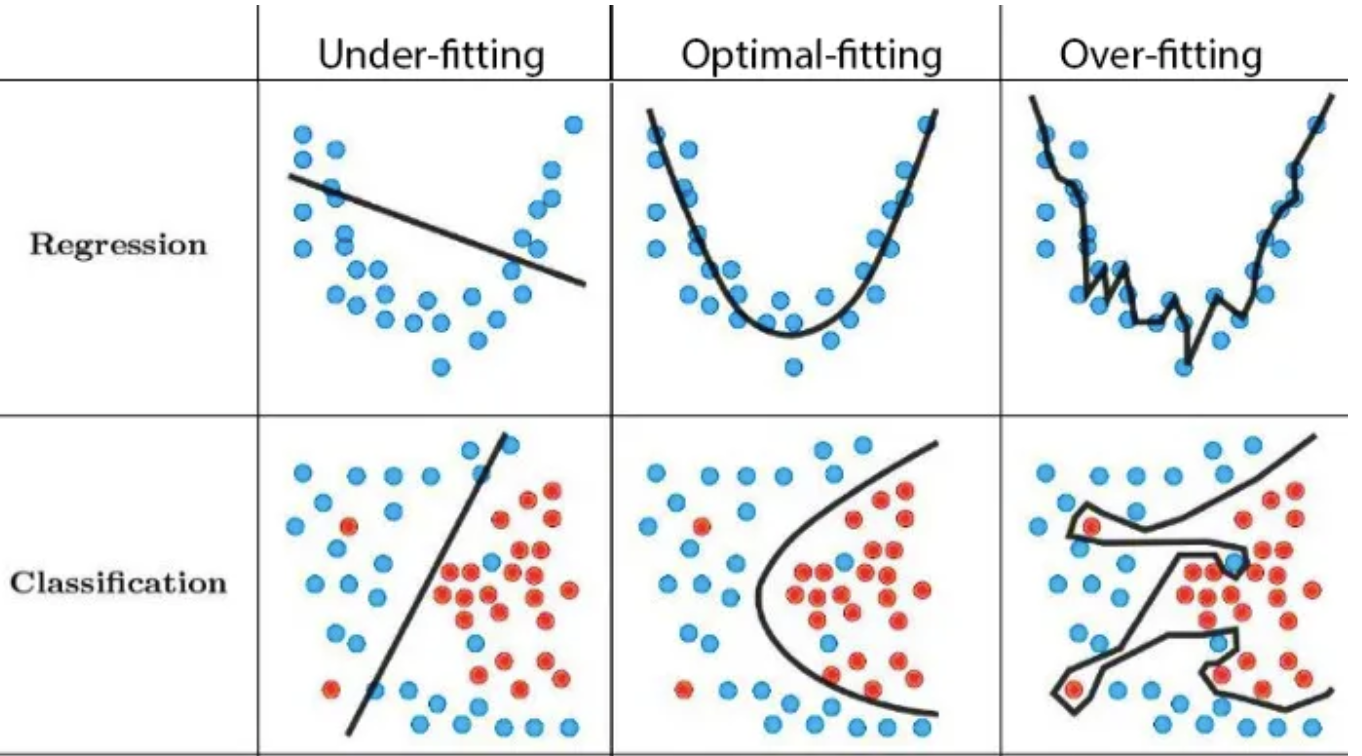
The fundamental tradeoff

Model	Training Score relative to Test Score	Performance
Too Complex	High training score compared to test score	Overfit
Too Simple	Low training score and low test score	Underfit

• Models that have extremely high training scores ahd have learned highly complex relationships in the training data can be overfit
• On the other hand, models that have low training scores and are very simple may not have learned the necessary relationships in the training data needed to predict well on unseen data; they are underfit

Sahu, P. (2020, September 9). Techniques for handling underfitting and overfitting in machine learning. Towards Data Science.

Empirical Risk Minimization (ERM)

• In ML we aim to minimize the empirical risk (the average loss over training data).
• The goal is to approximate the best possible model by minimizing the loss function on the training set.
• However, errors can occur at different stages of the learning process.

Three Main Errors

Approximation Error

• This error occurs when the model is too simple to capture the true underlying function.
• It represents the gap between the best possible model and the true function.
• Example: Using a linear model to fit a highly non-linear function.
• To minimize error (future lectures):
  • Use more complex models with higher capacity.
  • Apply feature engineering to capture more relevant information.

Estimation Error

• This error arises from the fact that we only have a finite sample of data.
• The model learned on the training data may not generalize well to unseen data.
• Small training data or sampling noise.
• Overfitting to the training data, leading to poor performance on unseen data.
• To minimize error (future lectures):
  • Increase the size of the training dataset.
  • Use regularization techniques to prevent overfitting.
  • Cross-validation for better model selection.

Optimization Error

• This error occurs when the algorithm fails to find the global minimum of the loss function during training.
• This can happen when the optimization process gets stuck in local minima or saddle points.
• To minimize error (future lectures):
  • Use more effective optimization algorithms (e.g., Adam, RMSprop).
  • Tune hyperparameters carefully.

Fundamental Trade-off

• Minimizing approximation error helps ensure that our model generalizes well to unseen data.

$$E_{approx} = (E_{test} - E_{train})$$

• There is often a trade-off between model complexity and test error:

  • A more complex model can fit the specific patterns in the training data, increasing $E_{approx}$.
  • This can lead to overfitting, where the model doesn't generalize well to new data.

• As model complexity increases, $E_{approx}$ tends to grow, making it harder for the model to generalize.

• However, more data can reduce $E_{approx}$ and improve generalization.

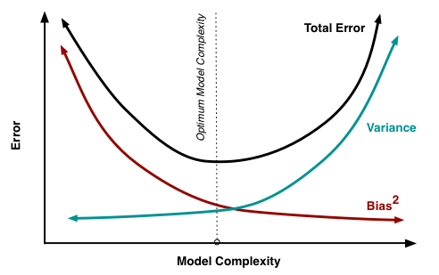
Bias-Variance Trade-off

• Bias error: Error due to incorrect assumptions in the learning model.

  • High bias leads to underfitting (the model fails to capture key patterns).

• Variance: Error due to the model's sensitivity to small fluctuations in training data.

  • High variance leads to overfitting (the model captures noise instead of the true signal).

• Key balance: The goal is to find the right balance between bias and variance for a model that generalizes well.

Cornell University. (2018). Lecture 12: Bias/Variance Tradeoff. Cornell University CS4780: Machine Learning.

Linear Regression

• Linear regression is one of the most basic and popular ML/statistical techniques.
• Used as a predictive model
• Assumes a linear relationship between the dependent variable (which is the variable we are trying to predict/estimate, y) and the independent variable/s (input variable/s used in the prediction, X)

Simple Linear Regression

• Only one independent/input variable is used to predict the dependent variable.

$$\hat{y} = wx + b$$

$\hat{y}$ = Dependent variable

$b$ = Constant

$w$ = Coefficients

$x$ = Independent variable

Multiple Linear Regression

• Many $x$'s and $w$'s

$$\hat{y} = w_1x_1 + w_2x_2 + ... + b$$

• The larger the value of $w_i$, the more influence $x_i$ has on the target $\hat{y}$

Matrix representation

• $\hat{y}$ is the linear function of features $x$ and weights $w$.

$$\hat{y} = w^Tx + b$$

• $\hat{y} \rightarrow$ prediction
• $w \rightarrow$ weight vector
• $b \rightarrow$ bias
• $x \rightarrow$ features

$$\hat{y} = \begin{bmatrix}w_1 & w_2 & \cdots & w_d\end{bmatrix}\begin{bmatrix}x_1 \\ x_2 \\ \vdots \\ x_d\end{bmatrix} + b$$

The Coffee-Productivity Dilemma: A Data-Driven Approach

Sarah is a team leader at a marketing firm. She has noticed a strange trend in her team's productivity. Some days, her team is incredibly efficient, completing projects ahead of schedule, while other days they struggle to meet even the simplest deadlines. After a few weeks of observation, Sarah notices that on days when her team seems especially productive, there are a lot more coffee cups piling up in the office trash bin.

Curious about the potential link between coffee consumption and work output, Sarah decides to investigate. She wonders, "Could there be a relationship between how much coffee my team drinks and their productivity (how many tasks are completed) throughout the day?"

import pandas as pd
import numpy as np
import matplotlib.pyplot as plt

Step 1: Load the data

df = pd.read_csv('data/coffee_productivity.csv', usecols = ['Coffee_Cups', 'Productivity'])
df.head()

	Coffee_Cups	Productivity
0	7	24.851737
1	4	12.687456
2	8	21.917630
3	5	19.208558
4	7	17.402905

Step 2: Identify the features X and the target y

X = df['Coffee_Cups'].values.reshape(-1, 1)
y = df['Productivity'].values

Step 3: Split into train and test sets.

• Using sklearn's train_test_split.
• It shuffles the data and then splits it.
• 80/20, 75/25, 70/30 are common splits.

from sklearn.model_selection import train_test_split

X_train, X_test, y_train, y_test = train_test_split(X, y, test_size=0.2, random_state=42)

Step 4: Choosing the model

Our problem's target is a numerical value. We need a regressor.

from sklearn.linear_model import LinearRegression
lr_sample = LinearRegression()
lr_sample.fit(X_train, y_train)

LinearRegression()

In a Jupyter environment, please rerun this cell to show the HTML representation or trust the notebook.
On GitHub, the HTML representation is unable to render, please try loading this page with nbviewer.org.

Step 5: Observe some of the outputs in the train set.

lr_sample.predict(X_train)[:5]

array([17.62058075, 20.11357862, 25.09957436, 12.634585  , 27.59257223])

y_train[:5]

array([18.7002218 , 23.09371016, 27.84047591,  9.24645982, 30.72015875])

Step 6: Observe some of the outputs in the test set.

lr_sample.predict(X_test)[:5]

array([17.62058075, 27.59257223, 20.11357862, 25.09957436, 12.634585  ])

y_test[:5]

array([16.21165539, 28.80351029, 23.433057  , 26.89351191, 13.10162284])

Step 7: Compare the scores

lr_sample.score(X_train, y_train)

0.8309714784972858

lr_sample.score(X_test, y_test)

0.82765549336117

fig, axes = plt.subplots(nrows=1, ncols=2, figsize=(14, 7))

axes[0].scatter(X_train, y_train, marker='o', s=2)
axes[0].set_title('Coffee vs Productivity', fontsize=16)
axes[0].set_xlabel('Cups of Coffee')
axes[0].set_ylabel('Productivity (completed tasks)')

axes[1].scatter(X_train, y_train, marker='o', alpha=0.5, s=2)
axes[1].plot(X_train, (lr_sample.coef_ * X_train) + lr_sample.intercept_, c='black')
axes[1].set_title('Coffee vs Productivity (with regression)', fontsize=16)
axes[1].set_xlabel('Cups of Coffee')
axes[1].set_ylabel('Productivity (completed tasks)')
axes[1].text(
    x=0.4,
    y=0.08,
    s='$\\hat{y}=-350.7x+7.7$',
    fontsize=18,
    fontweight='bold',
    transform=axes[1].transAxes
)

plt.show()

• The intuition behind Linear Regression is in the coefficients and intercept.

• Some literature refer to the coefficients as weights and the intercept as the bias. These are the parameters that are being learned during fit or training.

• In sklearn you can access them with the attributes .coef_ and .intercept_

lr_sample.coef_

array([2.49299787])

lr_sample.intercept_

np.float64(5.155591389534953)

Step 8: New observations

Sarah is interviewing new potential candidates for her team. In the interview she asks the following questions:

• How many cups of coffee do you drink in the morning?

She then gathers the following rows of data:

new_obs = pd.DataFrame({'Coffee_Cups': [4,5]})
new_obs

	Coffee_Cups
0	4
1	5

Step 9a: Calculation by Hand

# First person:
lr_sample.coef_*new_obs.loc[0, 'Coffee_Cups'] + lr_sample.intercept_

array([15.12758288])

# Second person:
lr_sample.coef_*new_obs.loc[1, 'Coffee_Cups'] + lr_sample.intercept_

array([17.62058075])

Step 9b: Calculation using sklearn .predict()

y_pred = lr_sample.predict(new_obs['Coffee_Cups'].values.reshape(-1, 1))
y_pred

array([15.12758288, 17.62058075])

Multivariable Regression

As Sarah digs deeper into the data, she begins to wonder, "Is coffee the only thing driving productivity? Could there be other factors at play?" One day, after observing that some team members seemed especially sluggish despite their high coffee intake, Sarah realizes that sleep might also be a factor.

Sarah decides to test her hypothesis. In addition to tracking coffee consumption, she starts asking her team to report their hours of sleep each day. Over the next month, Sarah records this new variable.

After collecting enough data, Sarah now has three columns:

1. Coffee consumption (cups per day).
2. Hours of sleep (hours per night).
3. Productivity (number of tasks achieved in the day).

df = pd.read_csv('data/coffee_productivity.csv')
df.head()

	Coffee_Cups	Hours_Sleep	Productivity
0	7	7.605595	24.851737
1	4	6.963707	12.687456
2	8	5.644447	21.917630
3	5	7.486539	19.208558
4	7	5.231440	17.402905

X = df.drop(columns=['Productivity'])
y = df['Productivity'].values

X_train, X_test, y_train, y_test = train_test_split(X, y, test_size=0.2, random_state=42)

Additional step: Scale the data so that it is comparable.

from sklearn.preprocessing import StandardScaler

scaler = StandardScaler()
X_train_scaled = scaler.fit_transform(X_train)

Important

Never do .fit_transform() on test data. Always use .transform() only.

X_test_scaled = scaler.transform(X_test)

lr = LinearRegression()
lr.fit(X_train_scaled, y_train)

LinearRegression()

In a Jupyter environment, please rerun this cell to show the HTML representation or trust the notebook.
On GitHub, the HTML representation is unable to render, please try loading this page with nbviewer.org.

lr_coeffs = lr.coef_
lr_coeffs

array([6.4249594 , 2.09152413])

lr_intercept = lr.intercept_
lr_intercept

np.float64(17.36193221782039)

words_coeffs_df = pd.DataFrame(data = lr_coeffs.T, index = X_train.columns, columns=['Coefficients'])
words_coeffs_df

	Coefficients
Coffee_Cups	6.424959
Hours_Sleep	2.091524

Why did we scale?

Sometimes variables are not really comparable. Scaling, allows us to put them in the same range. This allows us to be able to interpret the coefficients properly.

For interpreting linear models:

• if the coefficient is +, then if the feature value goes UP the predicted value goes UP
• if the coefficient is -, then if the feature values goes UP the predicted value goes DOWN
• if the coefficient is 0, the feature is not used in making a prediction.

Prediction

$$\hat{y} = w_1x_1 + w_2x_2 + ... + w_8x_8 + b$$

lr.predict(X_train_scaled)[:5]

array([15.53617259, 20.72490379, 28.2837986 , 10.5896231 , 27.82100943])

lr.predict(X_test_scaled)[:5]

array([17.23753722, 28.37399184, 22.42152222, 26.65615455, 13.31313734])

lr.intercept_ + (lr.coef_[0] * X_test_scaled[0][0]) + (lr.coef_[1] * X_test_scaled[0][1])

np.float64(17.237537221177554)

lr.score(X_train_scaled, y_train)

0.9192148183081769

lr.score(X_test_scaled, y_test)

0.9321424686508619

Linear Regression with statsmodels

import statsmodels.api as sm

model = sm.OLS(y_train, sm.add_constant(X_train_scaled))
results = model.fit()

results.params

array([17.36193222,  6.4249594 ,  2.09152413])

print(results.summary())

                            OLS Regression Results                            
==============================================================================
Dep. Variable:                      y   R-squared:                       0.919
Model:                            OLS   Adj. R-squared:                  0.919
Method:                 Least Squares   F-statistic:                     4534.
Date:                Tue, 22 Oct 2024   Prob (F-statistic):               0.00
Time:                        13:45:08   Log-Likelihood:                -1690.1
No. Observations:                 800   AIC:                             3386.
Df Residuals:                     797   BIC:                             3400.
Df Model:                           2                                         
Covariance Type:            nonrobust                                         
==============================================================================
                 coef    std err          t      P>|t|      [0.025      0.975]
------------------------------------------------------------------------------
const         17.3619      0.071    244.930      0.000      17.223      17.501
x1             6.4250      0.071     90.638      0.000       6.286       6.564
x2             2.0915      0.071     29.506      0.000       1.952       2.231
==============================================================================
Omnibus:                        0.145   Durbin-Watson:                   2.019
Prob(Omnibus):                  0.930   Jarque-Bera (JB):                0.143
Skew:                           0.032   Prob(JB):                        0.931
Kurtosis:                       2.989   Cond. No.                         1.00
==============================================================================

Notes:
[1] Standard Errors assume that the covariance matrix of the errors is correctly specified.

Score interpretation

• R-squared measures the proportion of the variation in your dependent variable (Y) explained by your independent variables (X) for a linear regression model

• Adjusted R-squared adjusts the statistic based on the number of independent variables in the model

• $R^2$ is a measure of fit.

• It indicates how much variation of a dependent variable is explained by the independent variables.

• An R-squared of 100% means that $y$ is completely explained by the independent variables.

$R^2 = 1 - \frac{Unexplained\:Variation}{Total\:Variation}$

$R^2 = 1 - \frac{RSS}{TSS}$

$R^2 = $ coefficient of determination
$RSS = $ sum of squares of residuals $ =\displaystyle\sum_{i=1}^{n}(y_{i}-{\hat{y}_{i}})^{2}$
$TSS = $ total sum of squares $ = \displaystyle\sum_{i=1}^{n}(y_{i}-\bar{y})^{2}$
$\bar{y}$ = mean value

Thus,

$ R^2 = 1 - \frac{\displaystyle\sum_{i=1}^{n}(y_{i}-{\hat{y}_{i}})^{2}}{\displaystyle\sum_{i=1}^{n}(y_{i}-\bar{y})^{2}} $

Going beyond linear regression: Polynomial regression

• Linear regression assumes a straight-line relationship between the variables.
• But what if the true relationship between the target (e.g., productivity) and the features (coffee cups and hours of sleep) is non-linear?
• Linear models can be limiting when the data follows a curve or more complex pattern.

Sarah's Coffee-Sleep-Productivity Example Revisited

• Sarah noticed that both coffee and sleep influence her team's productivity.
• However, as she collects more data, she realizes that productivity doesn't increase linearly with coffee or sleep.
• After a certain number of coffee cups, the productivity boost slows down.
• Too much or too little sleep seems to hurt productivity in a non-linear way.

What is Polynomial Regression?

• Polynomial regression extends linear regression by creating quadratic, cubic, and higher-order terms.
• We still use the linear regression framework, but we model more complex relationships by transforming the features.

Example:

• Instead of using just Coffee_Cups, we also use Coffee_Cups^2, Coffee_Cups^3, etc., to capture non-linear effects.

How Polynomial Regression Works:

• In addition to the original feature (Coffee_Cups), we create new features:

  • Coffee_Cups^2
  • Coffee_Cups^3

• These terms allow us to capture curves and more complex patterns.

• Our new model might look like: $$ \hat{y} = \beta_0 + \beta_1 x + \beta_2 x^2 + \beta_3 x^3 $$

• Key Takeaway: We can still use the linear regression framework by transforming our features into polynomial terms!

from sklearn.preprocessing import PolynomialFeatures

df = pd.read_csv('data/non_linear_coffee_productivity.csv')
df.head(2)

	Coffee_Cups	Hours_Sleep	Productivity
0	3	9.055615	11.421316
1	2	9.144187	6.674547

X = df.drop(columns=['Productivity'])
y = df['Productivity']

X_train, X_test, y_train, y_test = train_test_split(X, y, test_size=0.2, random_state=42)

# Create polynomial features (degree 2)
poly = PolynomialFeatures(degree=2)
X_poly_train = poly.fit_transform(X_train)

# Fit the polynomial regression model
model = LinearRegression()
model.fit(X_poly_train, y_train)

LinearRegression()

In a Jupyter environment, please rerun this cell to show the HTML representation or trust the notebook.
On GitHub, the HTML representation is unable to render, please try loading this page with nbviewer.org.

y_pred = model.predict(X_poly_train)

# We'll plot only the actual vs predicted productivity
plt.scatter(y_train, y_pred, color='blue', label='Predicted vs Actual')
plt.plot([min(y_train), max(y_train)], [min(y_train), max(y_train)], color='red', linestyle='--', label='Perfect Fit Line')
plt.xlabel('Actual Productivity (completed tasks)')
plt.ylabel('Predicted Productivity (completed tasks)')
plt.title('Polynomial Regression: Coffee, Sleep vs. Productivity')
plt.legend()
plt.show()

import plotly.graph_objects as go
import plotly.io as pio
pio.renderers.default = 'iframe'

scatter = go.Scatter3d(
    x=X_train['Coffee_Cups'], 
    y=X_train['Hours_Sleep'], 
    z=y_train,
    mode='markers',
    marker=dict(size=5, color='blue', opacity=0.8),
    name='Data'
)

surface = go.Mesh3d(
    x=X_train['Coffee_Cups'],
    y=X_train['Hours_Sleep'],
    z=y_pred,
    opacity=0.6,
    color='red',
    name='Polynomial Fit'
)

layout = go.Layout(
    title='Polynomial Regression: Coffee, Sleep vs. Productivity',
    scene=dict(
        xaxis_title='Cups of Coffee',
        yaxis_title='Hours of Sleep',
        zaxis_title='Productivity (completed tasks)',
        aspectratio=dict(x=1, y=1, z=1)
    )
)

fig = go.Figure(data=[scatter, surface], layout=layout)
fig.show()

What sklearn does is - if you substitute $x^2$ as another variable such as m, then the equation now is:

y=w*m + b

The relation between y and m is linear but it is not linear between x and y.

Because of this "technically", it is linear regression just the variables between which it happens is $x^2$ (m) and y and not x and y.